Paste data into excel. How to make a transfer in Excel in a cell. Paste Special: Divide and Multiply
We are all accustomed to the fact that we can copy and paste data from one cell to another using standard commands operating system Windows. To do this we need 3 keyboard shortcuts:
- Ctrl+C copying data;
- Ctrl+X cut out;
- Ctrl+V paste information from the clipboard.
So, Excel has a more advanced version of this feature.
Special insert is a universal command that allows you to paste copied data from one cell to another separately.
For example, you can paste separately from a copied cell:
- Comments;
- Cell Format;
- Meaning;
- Formula;
- Decor.
How Paste Special Works
First, let's find where the command is located. Once you've copied a cell, you can open Paste Special in several ways. You can right-click on the cell where you want to paste data and select “Paste Special” from the drop-down menu. In this case, you have the opportunity to use quick access to the insertion functions, and also by clicking on the link at the bottom of the list to open a window with all the possibilities. IN different versions This item may vary, so don't be alarmed if you don't have an additional drop-down menu.
You can also open a special insert on the tab home. At the very beginning, click on the special arrow, which is located under the button Insert.

The window with all the functions looks like this.

Now we’ll go through it in order and start with the “Insert” block.
- All- this is a common function that allows you to completely copy all cell data to a new location;
- Formulas- only the formula that was used in the copied cell will be transferred;
- Values- allows you to copy the result that is obtained during execution in a formula cell;
- Formats- only the cell format is transferred. Also, the cell design will be copied, for example, background fill;
- Notes- copying a cell note. In this case, the data (formula, values, etc.) is not copied;
- Conditions for values- using this option you can copy, for example, the criteria for acceptable data (drop-down list);
- With original theme- the cell is copied while maintaining the design. For example, if you use a background fill in a cell, that will be copied too. In this case, the formula will be copied;
- No frame- if a cell has a frame on either side, it will be deleted when copying;
- Column widths- the column width will be copied from one cell to another. This feature is very convenient to use when you are copying data from one sheet to another. Only column widths are transferred;
- Formulas and number formats- the formula and number format are transferred;
- Number values and formats- the result and number format are transferred.

Let's look at a few examples. There is a table in which the full name column is collected using the Concatenate function. We need to insert ready-made values instead of the formula.

To replace a formula with results:
- Copy the full name column;
- Right-click on the topmost cell and select Paste Special;
- Set the item to active Meaning and press the key OK.

Now the column contains the results instead of the formula.

Let's look at another example. To do this, copy and paste an existing table next to it.

As you can see, the table did not save the width of the columns. Our task now is to transfer the width of the columns to the new table.
- Copy the entire source table;
- Stand on the top left cell of the new table and right-click. Next, select Paste Special;
- Set the item to active Column widths and press the key OK.
Now the table looks exactly the same as the original one.

Now let's move on to the block Operations.
- Fold- the inserted information will be added to the values already in the cell;
- Subtract- the inserted information will be subtracted from the values already present in the cell;
- Multiply- the value in the cell will be multiplied by the inserted one;
- Divide- the value in the cell will be divided by the value being inserted.

Let's look at an example. There is a table in which there is a column with numerical values.

Task: multiply each number by 10. What you need to do to do this:
- In the new cell you need to put the number 10 and copy it to the clipboard;
- Select all the cells of the column in which we will multiply;
- Right-click on any of the selected cells and select Paste Special;
- Set it to active Multiply.

In the end we get the required result.

Let's consider one more problem. It is necessary to reduce the results obtained in the previous example by 20%.
- In the new cell we set 80% and copy it;
- Select all the cells of the column in which we will calculate the percentage;
- Right-click on any of the selected cells and select Paste Special;
- Set it to active Multiply.

As a result, we get values reduced by 20% from the original ones.

There is only one note here. When you work with a block Operations, try to display in a block Insert option Meaning, otherwise, when pasting, the formatting of the cell that we are pasting will be copied and the formatting that was originally there will be lost.

There are two last options left that can be activated at the bottom of the window:
- Skip empty cells- allows you not to paste empty cells from the copied range. The program will not erase data in a cell into which a blank cell is inserted;
- Transpose- changing the orientation of copied cells, i.e. rows become columns and columns become rows.

That's all, if you have any questions, be sure to ask them in the comments below.
Everyone knows the ability to copy and paste data through the operating system's Clipboard.
Hotkey combinations:
Ctrl+C - copy
Ctrl+X - cut
Ctrl+V - paste
Paste Special command - universal option Paste commands.
Paste special allows you to separately paste attributes of copied ranges. In particular, you can paste only comments, only formats, or only formulas from the copied range into a new location on the worksheet.
To make this command available, you must:
As a result, the Paste Special dialog box will appear on the screen, which will differ depending on the source of the copied data.
1. Inserting information from Excel
If you copied a range of cells in the same application, the Paste Special window will look like this:

Insert radio button group:
All - Selecting this option is equivalent to using the Paste command. This copies the cell contents and format.
Formulas - selecting this option allows you to paste only formulas as they were entered into the formula bar.
Values - selecting this option allows you to copy the results of calculations using formulas.
Formats - when using this option, only the format of the copied cell will be pasted into the cell or range.
Notes - if you need to copy only the notes for a cell or range, you can use this option. This option does not copy the cell's contents or its formatting attributes.
Value conditions - if a data validity criterion has been created for a specific cell (using the Data | Validation command), then this criterion can be copied to another cell or range using this option.
Without a border - there is often a need to copy a cell without a border. For example, if you have a table with a border, then when you copy the border cell, the border will also be copied. To avoid copying the frame, you can select this option.
Column Widths - You can copy column width information from one column to another.
Advice! This function is convenient to use when copying a finished table from one sheet to another.
Often after pasting a copied table into new leaf you have to adjust its size.
Sheet 1 Source table

Sheet 2 Insert

To avoid this, use the Column Widths insert. For this:
- Copy the original table.
- Go to a new sheet and select the cell to insert.
- Open the Paste Special dialog box, check the Column Widths option, and click OK.

As a result, you will receive an exact copy of the original table on a new sheet.
The skip empty cells option prevents the program from erasing the contents of cells in the paste area, which can happen if there are empty cells in the copied range.
The Transpose option changes the orientation of the copied range. Rows become columns and columns become rows. You can read more about this option in the Excel “Transpose” feature.
Switches from the Operation group allow you to perform arithmetic operations.
Let's look at examples of performing mathematical operations using the Paste Special dialog box.
Task 1. Add 5 to each value in cells A3:A12

- Enter the value “5” in any cell (in in this example- C1).
- Copy the value of cell C1.

- Select the range A3:A12 and open the Paste Special dialog box

4. Select the Fold operation and click OK.

As a result, all values in the selected range will be increased by 5.

Task 2. Reduce prices for goods in the range E4:E10 by 10% (without using formulas).

- Taking into account the discount, the new price will be 90% of the previous one, therefore, enter the value of 90% in any of the cells (in this example - F2).
- Let's copy the contents of cell F2 to the clipboard.
- Select the range E4:E10 and open the Paste Special dialog box
In this article we will show you a few more useful options that the tool is rich in. Special insert, namely: Values, Formats, Column Widths and Multiply/Divide. With these tools, you can customize your tables and save time on formatting and reformatting data.
If you want to learn how to transpose, remove references and skip empty cells using the tool Paste Special(Paste Special) Refer to the article Paste Special in Excel: Skip Blank Cells, Transpose and Remove References.
We insert only values
Let's take, for example, a spreadsheet that reports profits from cookie sales at a charity bake sale. You want to calculate how much profit was made in 15 weeks. As you can see, we used a formula that adds the amount of sales that was a week ago and the profit received this week. You see in the formula bar =D2+C3? Cell D3 shows the result of this formula – $100 . In other words, in the cell D3 value is displayed. And now comes the most interesting part! In Excel using the tool Paste Special(Paste Special) You can copy and paste the value of this cell without formula or formatting. This opportunity is sometimes vital, and I will show why later.
Suppose, after selling cookies for 15 weeks, you need to submit a general report on the results of the profit received. You may want to simply copy and paste the line that contains the grand total. But what happens if you do this?

Oops! Is this not at all what you expected? As you can see, the usual copy and paste action ended up copying only the formula from the cell? You need to copy and paste special the value itself. That's what we'll do! We use the command Paste Special(Paste Special) with parameter Values(Meanings) so that everything is done as it should.

Notice the difference in the image below.

Applying Special insert > Values, we insert the values themselves, not formulas. Great job!
You may have noticed something else. When we used the command Paste Special(Insert Special) > Values(Values), we have lost formatting. You see that the font is bold and number format(dollar signs) were not copied? You can use this command to quickly remove formatting. Hyperlinks, fonts, and number formats can be quickly and easily cleared, leaving you with just the values without any decorative stuff that might get in the way in the future. Great, right?
In fact, Special insert > Values is one of my favorite tools in Excel. It is vital! Often I am asked to create a table and present it at work or in community organizations. I'm always worried that other users might wreak havoc on the formulas I've entered. After I finish working with formulas and calculations, I copy all my data and use Paste Special(Insert Special) > Values(Values) on top of them. This way, when other users open my spreadsheet, the formulas can no longer be changed. It looks like this:

Note the contents of the cell's formula bar D3. There's no formula to it anymore =D2+C3, instead the value is written there 100 .
And one more very useful thing regarding the special insert. Let's say that in the table for accounting for profits from a charity cookie sale, I want to leave only the bottom line, i.e. delete all rows except week 15. See what happens if I just delete all these rows:

This annoying error appears #REF!(#LINK!). It appears because the value in this cell is calculated using a formula that refers to the cells above it. After we deleted these cells, the formula had nothing to refer to and reported an error. Use the commands instead Copy(Copy) and Paste Special(Insert Special) > Values(Values) on top of the original data (as we already did above), and then delete the extra rows. Great job:

Paste Special > Values: Highlights
- Select data
- Copy them. If the data is not copied, but cut, then the command Paste Special(Paste Special) will not be available, so be sure to use Copy.
- Select the cell where you want to paste the copied data.
- Click Paste Special(Special insert). It can be done:
- by right-clicking and selecting context menu Paste Special(Special insert).
- on the tab Home(Home), click the small triangle below the button Paste(Insert) and select from the drop-down menu Paste Special(Special insert).
- Check the option Values(Data).
- Click OK.
We insert only formats
Special insert > Formats this is another very useful tool in Excel. I like it because it makes it fairly easy to set up. appearance data. There are many uses for the tool Special insert > Formats, but I will show you the most remarkable. I think you already know that Excel is great for working with numbers and performing various calculations, but it is also great when you need to present information. Besides creating tables and counting values, you can do a variety of things in Excel, such as schedules, calendars, labels, inventory cards, and so on. Take a closer look at the templates that Excel offers when creating a new document:

I came across a pattern Winter 2010 schedule and I liked the formatting, font, color and design about it.

I don’t need the schedule itself, especially for the winter of 2010, I just want to remake the template for my purposes. What would you do if you were me? You can create a draft of the table and manually repeat the template design in it, but this will take a very long time. Or you can delete all the text in the template, but this will also take a lot of time. It's much easier to copy the template and make Paste Special(Insert Special) > Formats(formats) on a new sheet of your workbook. Voila!

Now you can enter data while maintaining all formats, fonts, colors and designs.

Paste Special > Formats: Highlights
- Select the data.
- Copy them.
- Select the cell where you want to paste data.
- Click Paste Special(Special insert).
- Check the option Formats(formats).
- Click OK.
Copy column widths to another sheet
Have you ever wasted a lot of time and effort circling around your spreadsheet trying to adjust the column sizes? My answer is of course yes! Especially when you need to copy and paste data from one table to another. Existing Settings column widths may not be suitable and even though automatic setting column width is handy tool, in some places it may not work as you would like. Special insert > Column widths is a powerful tool that should be used by those who know exactly what they want. Let's look at the list as an example best programs US MBA.

How could this happen? You can see how carefully the column width was adjusted to fit the data in the image above. I copied the top ten business schools and placed them on another sheet. Look what happens when we just copy and paste the data:

The content is inserted, but the column widths are far from appropriate. You want to get the exact same column widths as the original sheet. Instead of setting it manually or using auto-fit column width, just copy and paste Paste Special(Insert Special) > Column Widths(Column Widths) to the area where you want to adjust the column widths.


See how simple it is? Although this is a very simple example, you can already imagine how useful such a tool will be if Excel sheet contains hundreds of columns.
You can also adjust the width of empty cells to format them before manually entering text. Look at the columns E And F in the picture above. In the picture below I used the tool Special insert > Column widths to expand the columns. So, without any fuss, you can design your Excel sheet the way you want!

Paste Special > Column Widths: Key Points
- Select the data.
- Copy the selected data.
- Place the cursor on the cell whose width you want to adjust.
- Click Paste Special(Special insert).
- Check the option Column Widths(Column widths).
- Click OK.
Paste Special: Divide and Multiply
Remember our cookie example? Good news! A giant corporation found out about our charity event and offered to increase profits. After five weeks of sales, they will be donated to our charity, so the income will double (become twice as large) compared to what it was at the beginning. Let's go back to the table in which we kept track of the profits from the charity cookie sale, and recalculate the profits taking into account the new investments. I added a column showing that after five weeks of sales, profits will double, i.e. will be multiplied by 2 .

All income starting from the 6th week will be multiplied by 2 .To show new numbers, we need to multiply the corresponding column cells C on 2 . We can do this manually, but it will be much nicer if Excel does it for us using the command Paste Special(Insert Special) > Multiply(Multiply). To do this, copy the cell F7 and apply the command on the cells C7:C16. Totals have been updated. Great job!

As you can see, the tool Special insert > Multiply can be used in a variety of situations. The situation is exactly the same with Paste Special(Insert Special) > Divide(Divide). You can divide an entire range of cells by a specific number quickly and easily. You know what else? With help Paste Special(Insert Special) with option Add(Fold) or Subtract(Subtract) You can quickly add or subtract a number.
Paste Special > Divide/Multiply: Highlights
- Select the cell with the number you want to multiply or divide by.
- Copy the selected data.
- Place the cursor on the cells in which you want to perform multiplication or division.
- Click Paste Special(Special insert).
- Check the option Divide(Split) or Multiply(Multiply).
- Click OK.
So, in this tutorial you have learned some very useful features of the tool. Special insert, namely: learned to insert only values or formatting, copy column widths, multiply and divide data by given number, as well as adding and removing values directly from a range of cells.
Insert and delete rows, columns, and cells to optimize the layout of your worksheet.
Note: IN Microsoft Excel The row and column limits are as follows: 16,384 columns wide by 1,048,576 rows high.
Inserting and deleting a column
To insert a column, select it and then on the tab home click the button Insert and select Insert columns into a sheet.
To remove a column, select it and then on the tab home click the button Insert and select Remove columns from a sheet.
You can also right-click at the top of the column and select Insert or Delete.
Inserting and deleting a row
To insert a row, select it, and then on the tab home click the button Insert and select Insert rows into a sheet.
To delete a row, select it, and then on the tab home click the button Insert and select Remove rows from a sheet.
You can also right-click the highlighted line and select the command Insert or Delete.
Inserting a cell
Select one or more cells. Right click and select command Insert.
In the window Insert select the row, column, or cell to insert.
For example, to insert a new cell between the Summer and Winter cells:
Click the Winter cell.
On the tab home Insert and select a team Insert Cells (Shift Down).

New cell is added above the "Winter" cell:

Inserting Rows
To insert one row: Right-click the entire line you want to insert a new line above and select Insert rows.

To insert multiple rows, follow these steps: Select the same number of rows above which you want to add new ones. Right-click the selection and select Insert rows.
inserting columns
To insert one new column, follow these steps: Right-click the entire column to the right of where you want to add the new column. For example, to insert a column between columns B and C, right-click column C and select Insert columns.

To insert multiple columns, follow these steps: Select the same number of columns to the right of which you want to add new ones. Right-click the selection and select Insert Columns.
Delete cells, rows, and columns
If you no longer need any cells, rows, or columns, here's how to delete them:
Select the cells, rows, or columns you want to delete.
On the tab home click the arrow below the button Delete and select the desired option.

When you delete rows or columns, the following rows and columns are automatically moved up or to the left.
Advice: If you change your mind right after you delete a cell, row, or column, simply press CTRL+Z to restore it.
A drop-down list in Excel is perhaps one of the most convenient ways to work with data. You can use them both when filling out forms and creating dashboards and voluminous tables. Drop-down lists are often used in applications on smartphones and websites. They are intuitive for the average user.
Click the button below to download a file with examples of drop-down lists in Excel:
Video tutorial
How to create a drop-down list in Excel based on data from the list
Let's imagine that we have a list of fruits:
To create a dropdown list we will need to do the following steps:
- Go to the “tab” Data” => section “ Working with data ” on the toolbar => select the item “ Data checking “.
- In the pop-up window “ Validation of entered values ” on the “ tab Options” in the data type select “ List “:
- In field " Source” enter a range of fruit names =$A$2:$A$6 or simply place the mouse cursor in the value entry field “ Source” and then select the data range with the mouse:
If you want to create dropdown lists in multiple cells at a time, then select all the cells in which you want to create them and then follow the steps above. It is important to ensure that cell references are absolute (for example, $A$2), rather than relative (for example, A2 or A$2 or $A2 ).
How to make a dropdown list in Excel using manual data entry
In the example above, we entered a list of data for a drop-down list by selecting a range of cells. In addition to this method, you can enter data to create a drop-down list manually (it is not necessary to store it in any cells).
For example, imagine that we want to display two words “Yes” and “No” in a drop-down menu. For this we need:
- Select the cell in which we want to create a drop-down list;
- Go to the “tab” Data” => section “ Working with data ” on the toolbar => select “ Data checking “:
- In the pop-up window “ Validation of entered values ” on the “ tab Options” in the data type select “ List “:
- In field " Source” enter the value “Yes; No".
- Click “ OK “
The system will then create a drop-down list in the selected cell. All items listed in the “ Source“, separated by semicolons, will be reflected in different lines of the drop-down menu.
If you want to simultaneously create a drop-down list in several cells, select the required cells and follow the instructions above.
How to create a drop-down list in Excel using the OFFSET function
Along with the methods described above, you can also use a formula to create drop-down lists.
For example, we have a list with a list of fruits:
In order to make a drop-down list using a formula, you need to do the following:
- Select the cell in which we want to create a drop-down list;
- Go to the “tab” Data” => section “ Working with data ” on the toolbar => select “ Data checking “:
- In the pop-up window “ Validation of entered values ” on the “ tab Options” in the data type select “ List “:
- In field " Source”enter the formula: =OFFEST(A$2$,0,0,5)
- Click “ OK “
The system will create a drop-down list with a list of fruits.
How does this formula work?
In the example above we used the formula = OFFSET(link, row_offset, column_offset, [height], [width]).
This function contains five arguments. In the argument “ link” (in the example $A$2) indicates which cell to start shifting from. In arguments “offset_by_rows" And “offset_by_columns”(in the example the value is “0”) – how many rows/columns need to be shifted to display the data. In the argument “ [height]” the value “5” is specified, which indicates the height of the range of cells. Argument “ [width]” we do not indicate, since in our example the range consists of one column.
Using this formula, the system returns to you as data for the dropdown list a range of cells starting with cell $A$2, consisting of 5 cells.
How to make a drop-down list in Excel with data substitution (using the OFFSET function)
If you use the formula in the example above to create a list, you are creating a list of data captured in a specific range of cells. If you want to add any value as a list item, you will have to adjust the formula manually. Below you will learn how to make a dynamic drop-down list that will automatically load new data for display.
To create a list you will need:
- Select the cell in which we want to create a drop-down list;
- Go to the “tab” Data” => section “ Working with data ” on the toolbar => select “ Data checking “;
- In the pop-up window “ Validation of entered values ” on the “ tab Options” in the data type select “ List “;
- In field " Source”enter the formula: =OFFEST(A$2$,0,0,COUNTIF($A$2:$A$100;”<>”))
- Click “ OK “
In this formula, in the argument “[ height]” we specify as an argument denoting the height of the list with data - a formula that calculates in a given range A2:A100 number of non-empty cells.
Note: For correct operation formulas, it is important that there are no empty lines in the list of data to be displayed in the drop-down menu.
How to create a drop-down list in Excel with automatic data substitution
In order for new data to be automatically loaded into the drop-down list you created, you need to do the following:
- We create a list of data to display in the drop-down list. In our case, this is a list of colors. Select the list with the left mouse button:
- On the toolbar, click “ Format as table “:

- From the drop-down menu, select the table design style:

- By pressing the “ OK” in the pop-up window, confirm the selected range of cells:
- Then, select the table data range for the drop-down list and give it a name in the left margin above column “A”:
The table with the data is ready, now we can create a drop-down list. To do this you need:
- Select the cell in which we want to create a list;
- Go to the “tab” Data” => section “ Working with data ” on the toolbar => select “ Data checking “:
- In the pop-up window “ Validation of entered values ” on the “ tab Options” in the data type select “ List “:
- In the source field we indicate =”name of your table” . In our case, we called it “ List “:

- Ready! A drop-down list has been created, it displays all the data from the specified table:

- In order to add a new value to the drop-down list, simply add information to the cell next after the table with the data:

- The table will automatically expand its data range. The drop-down list will be replenished accordingly with a new value from the table:

How to copy a dropdown list in Excel
Excel has the ability to copy created drop-down lists. For example, in cell A1 we have a dropdown list that we want to copy to a range of cells A2:A6 .
To copy a drop-down list with the current formatting:
- left-click on the cell with the drop-down list that you want to copy;
- CTRL+C ;
- select cells in a range A2:A6, where you want to insert the dropdown list;
- press the keyboard shortcut CTRL+V .
So, you will copy the drop-down list, maintaining the original list format (color, font, etc.). If you want to copy/paste a dropdown list without saving the format, then:
- left-click on the cell with the drop-down list that you want to copy;
- press the keyboard shortcut CTRL+C ;
- select the cell where you want to insert the drop-down list;
- right-click => bring up the drop-down menu and click “ Special insert “;
- In the window that appears, in the “ Insert” select item “ conditions for values “:
- Click “ OK “
After this, Excel will copy only the data from the drop-down list, without preserving the formatting of the original cell.
How to select all cells containing a drop-down list in Excel
Sometimes it is difficult to understand how many cells are in Excel file contain drop-down lists. There is an easy way to display them. For this:
- Click on the “ tab home” on the Toolbar;
- Click “ Find and highlight ” and select “ Select a group of cells “:
- In the dialog box, select “ Data checking “. In this field you can select the items “ Everyone" And " These same “. “Everyone” will allow you to select all drop-down lists on the sheet. Paragraph " these same” will show drop-down lists with similar data content in the drop-down menu. In our case we choose “ everyone “:
Read also...
- Cadaques in Spain. My review and photo. Cadaques, Catalonia Cadaques Spain how to get there from Barcelona
- Shopping cart for an online store at the front or Writing modular javascript
- Falling snow on jQuery or html New Year greeting card template
- Where to see what version of Android is installed on an Honor and Huawei phone How to find out the Huawei serial number