How can you format a table in excel. TOP hotkeys for working in Excel
The most vivid and memorable event that I remember and which has gone down in history is the referendum that took place in Crimea. We were very pleased with the results of this referendum. I remember this day, March 16, 2014. Me and all my relatives hurried to the polling stations to vote for Crimea to join the Russian Federation. Smiling people walked the streets, and grandparents were especially happy. It was a holiday for them; they went to the polling stations with flowers. On May 18, all people gathered in the central squares of cities in order to hear the results of this referendum. Everyone sincerely believed that the results would be positive. She did just that. People were happy. They said that they had returned to their homeland. At the same time, there was fear in the air. Fear that there will be a war, since the Ukrainian authorities may not accept the result. But despite all this, there was a holiday for the people.
Recent political events that have upset
- events on the Maidan in Kyiv 2013-2014;
- events in Odessa 2014;
- war in Donbass.
Among the political events that I am very saddened by, I would like to include the events that preceded the Crimean Spring, namely, the referendum in Crimea in 2014. Namely, this is the horror that happened on the Maidan in Kyiv. How they mocked Berkut, and there were young guys there. They prayed every day to survive. This is also the horror that happened in Odessa. There are simply no words to describe this. This is not a human act when they burned people alive in the house of trade unions. It's terrible, when we heard or saw this on the news, tears flowed. It was impossible to contain them. Another terrible event is the military operations in Donbass. Many familiar people who lived in that territory fled to Crimea. And when communicating with friends who live there, we worried about them, praying that nothing would happen to them. Another terrible event was the attacks on buses with people who opposed the Maidan. Our friends and neighbors were on these buses. And when we heard from them what was happening there, we simply could not find the words to say anything. The only good thing is that it's over.
Excel is needed to create tables and make calculations. Now we will learn how to correctly compile and format tables.
Open Excel (Start - Programs - Microsoft Office- Microsoft Office Excel).
At the top there are buttons for editing. This is what they look like in Microsoft Excel 2003:
And so - in Microsoft Excel 2007-2016:
After these buttons there is the working (main) part of the program. It looks like one big table.

Each of its cells is called a cell.
Pay attention to the topmost cells. They are highlighted in a different color and called A, B, C, D and so on.
In fact, these are not cells, but column names. That is, it turns out that we have a column with cells A, a column with cells B, a column with cells C, and so on.
Also pay attention to the small rectangles with the numbers 1, 2, 3, 4, etc. on the left side of Excel. These are also not cells, but row names. That is, it turns out that the table can also be divided into rows (line 1, line 2, line 3, etc.).
Based on this, each cell has a name. For example, if I click on the first cell from the top left, then you can tell that I clicked on cell A1 because it is in column A and row 1.

And in the next picture, cell B4 is clicked.

Please note that when you click on a particular cell, the column and row in which they are located changes color.
Now let's try to print some numbers in B2. To do this you need to click on this cell and type numbers on the keyboard.

To consolidate the entered number and move to the next cell, press the Enter button on your keyboard.
By the way, there are a lot of cells, rows and columns in Excel. You can fill out the table ad infinitum.
Design Buttons in Excel
Let's look at the design buttons at the top of the program. By the way, they are also available in Word.
Font. The style in which the text will be written.
Letter size
Style (bold, italic, underlined)
Using these buttons you can align text in a cell. Place it on the left, center or right.
By clicking on this button, you can cancel the previous action, that is, go back one step.
Change text color. To select a color, you need to click on the small arrow button.
Using this button you can fill the cell with color. To select a color you need to click on the small arrow button.
How to create a table in Excel
Look at the small table already compiled in Excel:

Its upper part is the hat.
In my opinion, making the header is the most difficult part of creating a table. We need to think through all the points and provide for a lot. I advise you to take this seriously, because very often, due to an incorrect header, you have to redo the entire table.
Following the header is the content:
And now in practice we will try to compose in Excel program such a table.
In our example, the header is the top (first) line. Usually that's where she is.
Click on cell A1 and type the first item “Name”. Then click in cell B1 and type the next item - “Quantity”. Please note that words do not fit in cells.

Fill in the remaining cells C1 and D1.

Now let’s bring the hat back to normal. First you need to expand the cells, or rather the columns in which the words do not fit.
To expand a column you need to move the cursor (mouse arrow) over the line separating the two columns, in our case, the line between A and B. The cursor will change and take the form of an unusual double-sided black arrow. Click left button mouse and, without releasing it, stretch the column to the desired width.

The same can be done with strings.
To expand a string Place the cursor (mouse arrow) on the line separating the two lines. The cursor will change and take the form of an unusual double-sided black arrow. Press the left mouse button and, without releasing it, stretch the line to the desired width.

Expand the columns where the text does not fit. Then make the hat a little bigger. To do this, move the cursor over the line between lines 1 and 2. When it changes view, press the left button and, without releasing it, expand the first line.
It is customary for the header to be slightly different from the content. In the table we are repeating, the header items are “thicker” and “blacker” than the rest of the content, as well as the cells are shaded gray. To do this, you need to use the top part of Excel.
Click cell A1. With this simple action you will select it, that is, you will “tell” Excel that you are going to change something in this cell. Now click on the button at the top of the program. The text in the cell will become thicker and blacker (bold).
Of course, you can change the remaining points in the same way. But imagine that we have not four of them, but forty-four... This will take a lot of time. To make this faster, we need to select the part of the table that we are going to change. In our case, this is the header, that is, the first line.
There are several ways to highlight.
Selecting an entire Excel table. To do this, click on the small rectangular button in the left corner of the program, above the first line (the rectangle with the number 1).

Selecting part of a table. To do this, click on the cell with the left mouse button and, without releasing it, circle the cells that you want to select.
Select a column or row. To do this, click on the name of the desired column
or strings
By the way, you can select several columns and rows in the same way. To do this, click on the name of the column or row with the left mouse button and, without releasing it, drag along the columns or rows that you want to select.

Now let's try to change the header of our table. To do this, select it. I suggest selecting the entire line, that is, clicking on the number 1.
After this, we will make the letters in the cells thicker and blacker. To do this, press the button
Also in the table we need to make, the words in the header are located in the center of the cell. To do this, click the button
Well, finally, let’s paint the cells in the header light gray. To do this, use the button
To select the appropriate color, click on the small button next to it and select the desired one from the list of colors that appears.

We did the hardest thing. All that remains is to fill out the table. Do it yourself.
And now the final touch. Let's change the font and size of letters in the entire table. Let me remind you that first we need to select the part that we want to change.
I suggest selecting the entire table. To do this, click the button
Well, let's change the font and size of the letters. Click on the small arrow button in the field that is responsible for the font.
Select a font from the list that appears. For example, Arial.
By the way, there are a lot of fonts in programs from the Microsoft Office suite. True, not all of them work with the Russian alphabet. You can make sure that there are a lot of them by clicking on the small arrow button at the end of the field to select a font and scrolling the wheel on the mouse (or moving the slider on the right side of the window that appears).
Then change the size of the letters. To do this, click on the small button in the field indicating the size and select the desired one from the list (for example, 12). I remind you that the table must be selected.
If suddenly the letters no longer fit into the cells, you can always expand the column, as we did at the beginning of compiling the table.
And one more very important point. In fact, the printed table we compiled will have no borders (no partitions). It will look like this:

If you are not satisfied with this “limitless” option, you must first select the entire table, and then click on the small arrow at the end of the button, which is responsible for the borders.
From the list, select "All borders".
![]()
If you did everything correctly, you will get a table like this.
Tables in Excel are a series of rows and columns of related data that you manage independently of each other.
Working with tables in Excel, you can create reports, make calculations, build graphs and charts, sort and filter information.
If your job involves data processing, then knowing how to work with Excel tables will help you save a lot of time and increase efficiency.
How to work with tables in Excel. Step-by-step instruction
Before working with tables in Excel, follow these recommendations for organizing data:
- Data should be organized in rows and columns, with each row containing information about one record, such as an order;
- The first row of the table should contain short, unique headings;
- Each column must contain one type of data, such as numbers, currency, or text;
- Each row should contain data for one record, such as an order. If applicable, provide a unique identifier for each line, such as an order number;
- The table should not have empty rows and absolutely empty columns.
1. Select an area of cells to create a table
Select the area of cells in which you want to create a table. Cells can be either empty or with information.
2. Click the “Table” button on the Quick Access Toolbar
On the Insert tab, click the Table button.
3. Select a range of cells
In the pop-up, you can adjust the location of the data and also customize the display of headings. When everything is ready, click “OK”.
4. The table is ready. Fill in the data!
Congratulations, your table is ready to be filled out! You will learn about the main features of working with smart tables below.
Pre-configured styles are available to customize the table format in Excel. All of them are located on the “Design” tab in the “Table Styles” section:
If 7 styles are not enough for you to choose from, then by clicking on the button in the lower right corner of table styles, all available styles will open. In addition to the styles preset by the system, you can customize your format.
In addition to the color scheme, in the table “Designer” menu you can configure:
- Show header row – enables or disables headers in the table;
- Total line – enables or disables the line with the sum of the values in the columns;
- Alternating lines – highlights alternating lines with color;
- First column – makes the text in the first column with data “bold”;
- Last Column – makes the text in the last column “bold”;
- Alternating columns – highlights alternating columns with color;
- Filter Button – Adds and removes filter buttons to column headers.
How to add a row or column to an Excel table
Even within an already created table, you can add rows or columns. To do this, right-click on any cell to open a pop-up window:
- Select “Insert” and left-click on “Table Columns on the Left” if you want to add a column, or “Table Rows Above” if you want to insert a row.
- If you want to delete a row or column in a table, then go down the list in the pop-up window to the “Delete” item and select “Table Columns” if you want to delete a column or “Table Rows” if you want to delete a row.
How to sort a table in Excel
To sort information when working with a table, click the “arrow” to the right of the column heading, after which a pop-up window will appear:
In the window, select the principle by which to sort the data: “ascending”, “descending”, “by color”, “numeric filters”.
To filter information in the table, click the arrow to the right of the column heading, after which a pop-up window will appear:
- “Text filter” is displayed when there are text values among the column data;
- “Filter by color”, just like a text filter, is available when the table has cells painted in a color different from the standard design;
- “Numerical filter” allows you to select data by parameters: “Equal to...”, “Not equal to...”, “Greater than...”, “Greater than or equal to...”, “Less than...”, “Less than or equal to...”, “Between...”, “Top 10...”, “Above average”, “Below average”, and also set up your own filter.
- In the pop-up window, under “Search”, all data is displayed, by which you can filter, and with one click, select all values or select only empty cells.
If you want to cancel all filtering settings you have created, open the pop-up window above the desired column again and click “Remove filter from column”. After this, the table will return to its original form.
How to calculate a sum in an Excel table

In the window list, select “Table” => “Total Row”:

A subtotal will appear at the bottom of the table. Left-click on the cell with the amount.
In the drop-down menu, select the principle of the subtotal: it can be the sum of the column values, “average”, “quantity”, “number of numbers”, “maximum”, “minimum”, etc.
How to fix a table header in Excel
The tables you have to work with are often large and contain dozens of rows. Scrolling down a table makes it difficult to navigate the data if the column headings are not visible. In Excel, you can attach a header to a table so that when you scroll through the data, you will see the column headings.
To fix headers, do the following:
- Go to the “View” tab in the toolbar and select “Freeze Panes”:
- Select “Freeze top row”: